Zoomed maps with ggforce!

I was recently asked via twitter to share some code on how I implemented the facet_zoom() function, from the newly released ggforce package, to zoom in on a particular region of a map. I’ve no idea if this is the “best” way of creating these sorts of maps, but anyway, here goes…

This way of making maps requires a number of packages, so make sure you have these installed first, then load them like so…

library(mapdata)
library(maptools)
library(raster)
library(rgeos)
library(ggplot2)
library(ggforce)
library(ggsn)

Our first step is to source the data that will form our map’s base layer. This comes from the mapdata package, and we will need the worldHires data. You’ll get an automatic graphical output which should be a map of the world.

mapBase <- map("worldHires", fill = T)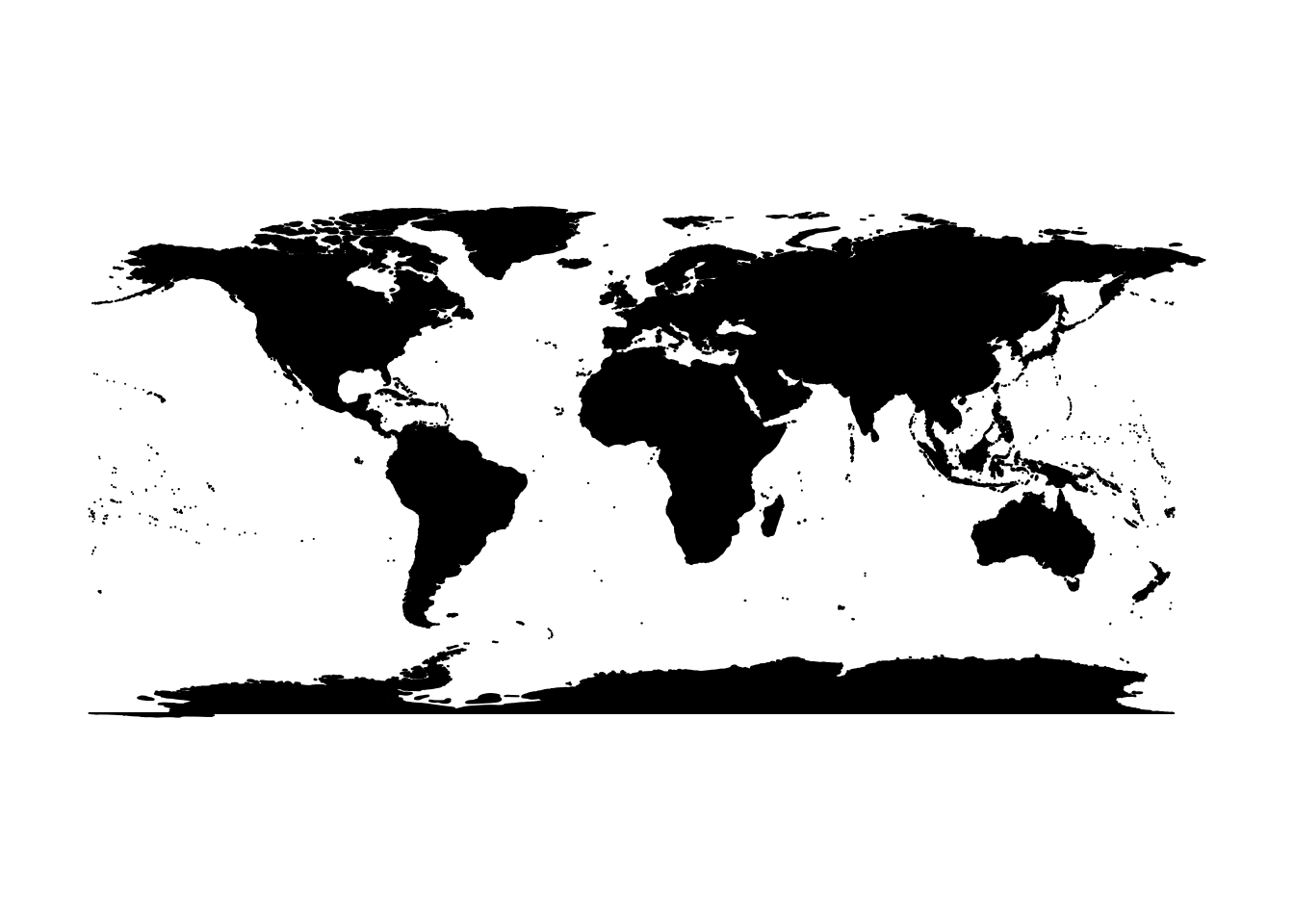

We now need to manipulate these data a bit to go from a map class object, to a SpatialPolygons object, which we can use with R’s GIS capabilities.

# first extract the IDs of what will be each spatial polygon
ids <- sapply(strsplit(mapBase$names, ":"), function(x) tail(x, n = 1))

# then, coerce map to spatial polygons object
mapPoly <- map2SpatialPolygons(mapBase, IDs = ids,
    proj4string = CRS("+proj=longlat +datum=WGS84"))

Next, we need to create an extent object to limit the spatial polygons to the region we are interested in plotting. The extent object will also need to share the same projection as the spatial polygons object. The coordinates in the extent call are given in the form Xmin, Xmax, Ymin, Ymax.

# create an extent and coerce to spatial polygon class
mapExtent <- as(extent(-20, 60, -40, 60), "SpatialPolygons")

# change projection to match the spatial polygon map
proj4string(mapExtent) <- CRS(proj4string(mapPoly))

Now we use the gBuffer and gIntersection functions to clip the spatial polygon map down to our region of interest. The 0 width buffer applied helps mop up topology errors with polygons self-intersecting.

buffMap <- gBuffer(mapPoly, byid = TRUE, width = 0)
cropMap <- gIntersection(buffMap, mapExtent, byid = TRUE)

Phew, that’s all the nasty GIS stuff dealt with. The rest is fairly standard data manipulation, then making the map look pretty and informative.

ggplot is unable to deal with many spatial data formats, so we need to turn it into something it can read, a data.frame.

mapDf <- fortify(cropMap, region = "id")

Now let’s simulate some points to plot onto our map.

locations <- data.frame(lat = runif(25, -40, 60),
  long = runif(25, -20, 60))

We now have enough to make a basic, but effective map.

ggplot() +
  geom_map(map = mapDf, data = mapDf, aes(x = long, y = lat, map_id = id),
    fill = "lightgrey", color = "lightgrey") +
  geom_point(data = locations, aes(x = long, y = lat, group = NULL))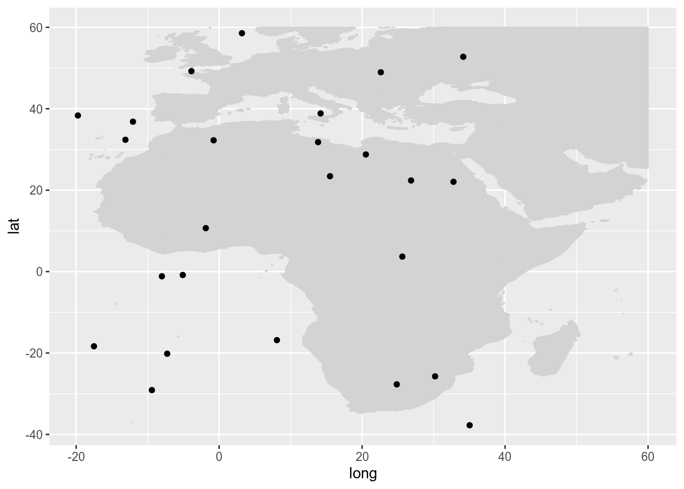

Not bad, but we can do better. The background is annoying and needs to go, the points could be made bigger and clearer, and don’t forget to add a scalebar! Also, say there are lots of points in one region that we want to zoom in on, we could use the facet_zoom function to get a closer look at those points.

In order to use facet_zoom, we need to create a factor level in the locations data that we can use to subset the data. Here, I want to zoom in on all points with a longitude and latitude greater than 20, so I need to create a factor which reflects this.

locations$region <- ifelse(locations$lat > 20 & locations$long > 20, 1, 2)
# this designates all points in my region of interest as 1's, and
# points outside the region are 2's

Now to tidy up our map.

ggplot() +
  geom_map(map = mapDf, data = mapDf, aes(x = long, y = lat, map_id = id),
    fill = "lightgrey", color = "lightgrey") +
  geom_point(data = locations, aes(x = long, y = lat, group = NULL),
    size = 2.5) +
  ggsn::scalebar(data = mapDf, dist = 2000, model = "WGS84", st.size = 5,
    anchor = c(x = 55, y = -40), transform  = T, dist_unit = "km") +
  facet_zoom(xy = region == 1, zoom.size = 1) +
  labs(x = "Latitude (decimal degrees)", y = "Longitude (decimal degrees)") +
  theme_bw() +
  theme(axis.text = element_text(size = 16),
    axis.title = element_text(size = 18),
    panel.grid.minor = element_blank(),
    panel.grid.major = element_blank())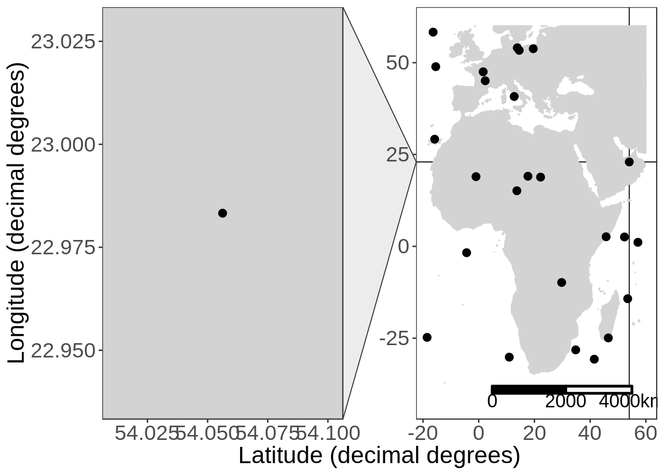

Depending on the dimensions of your zoomed in region, you may want to play around with the zoom.size parameter to get the right aspect ratio. But there you have it, combining ggforce with ggplot2 to make lovely looking maps!