Speeding up rarefaction curves for microbial community ecology

When beginning analyses on microbial community data, it is often helpful to compute rarefaction curves. A rarefaction curve tells you about the rate at which new species/OTUs are detected as you increase the number of individuals/sequences sampled. It does this by taking random subsamples from 1, up to the size of your sample, and computing the number of species present in each subsample. Ideally, you want your rarefaction curves to be relatively flat, as this indicates that additional sampling would not likely yield further species.

The vegan package in R has a nice function for computing rarefaction curves for species by site abundance tables. However, for microbial datasets this function is often prohibitively slow. This is due to the fact that we often have large numbers of samples, and each sample may contain several thousand sequences, meaning that a large number of random subsamples are taken.

Part of the problem is that the original function only makes use of a single processing core, meaning that random subsamples are computed serially, and each sample is processed serially. This means we could speed the function up by splitting samples across multiple cores. In short, we are parallelising the function.

Below is my attempt to modify the original code into a function that can use multiple processor cores to speed up the calculations.

# you will need to install the parallel package before hand
# and the vegan package if you dont have it
library(vegan)
quickRareCurve <- function (x, step = 1, sample, xlab = "Sample Size",
  ylab = "Species", label = TRUE, col, lty, max.cores = T, nCores = 1, ...)
{
    require(parallel)
    x <- as.matrix(x)
    if (!identical(all.equal(x, round(x)), TRUE))
        stop("function accepts only integers (counts)")
    if (missing(col))
        col <- par("col")
    if (missing(lty))
        lty <- par("lty")
    tot <- rowSums(x) # calculates library sizes
    S <- specnumber(x) # calculates n species for each sample
    if (any(S <= 0)) {
        message("empty rows removed")
        x <- x[S > 0, , drop = FALSE]
        tot <- tot[S > 0]
        S <- S[S > 0]
    } # removes any empty rows
    nr <- nrow(x) # number of samples
    col <- rep(col, length.out = nr)
    lty <- rep(lty, length.out = nr)
    # parallel mclapply
    # set number of cores
    mc <- getOption("mc.cores", ifelse(max.cores, detectCores(), nCores))
    message(paste("Using ", mc, " cores"))
    out <- mclapply(seq_len(nr), mc.cores = mc, function(i) {
        n <- seq(1, tot[i], by = step)
        if (n[length(n)] != tot[i])
            n <- c(n, tot[i])
        drop(rarefy(x[i, ], n))
    })
    Nmax <- sapply(out, function(x) max(attr(x, "Subsample")))
    Smax <- sapply(out, max)
     plot(c(1, max(Nmax)), c(1, max(Smax)), xlab = xlab, ylab = ylab,
       type = "n", ...)
    if (!missing(sample)) {
      abline(v = sample)
      rare <- sapply(out, function(z) approx(x = attr(z, "Subsample"),
         y = z, xout = sample, rule = 1)$y)
      abline(h = rare, lwd = 0.5)
      }
    for (ln in seq_along(out)) {
      N <- attr(out[[ln]], "Subsample")
      lines(N, out[[ln]], col = col[ln], lty = lty[ln], ...)
      }
    if (label) {
      ordilabel(cbind(tot, S), labels = rownames(x), ...)
      }
    invisible(out)
}

Most of the code is verbatim to the original, but you’ll notice a few extra arguments to specify, and a few extra lines that determine how many cores the function will use.

Essentially, if you do not specify a number of cores, the function will default to using all available cores, which will allow the quickest calculation. Otherwise, you can specify max.cores = F, which will allow you to specify the number of cores using nCores. This is handy if you need some cores to remain usable whilst running the function.

Below is a usage example.

# load some dummy data
data(dune)

quickRareCurve(dune) # will use all cores and print how many cores you have

quickRareCurve(dune, max.cores = F, nCores = 2) # use only 2 cores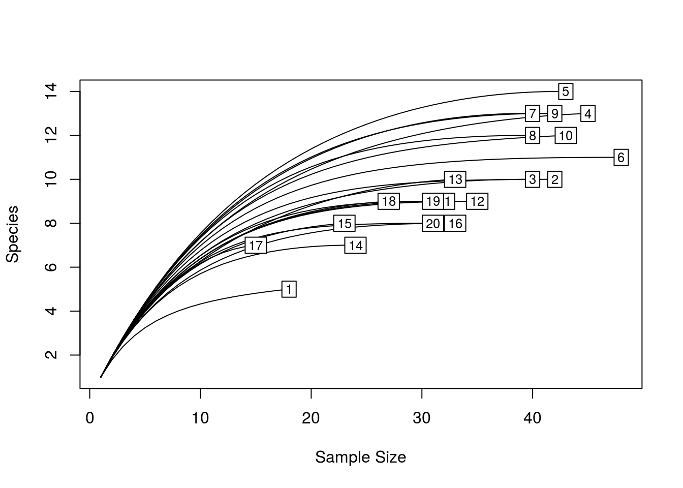

We can compare the new function’s performance to the original using the microbenchmark package, as below.

library(microbenchmark)

microbenchmark(rarecurve(dune), quickRareCurve(dune), times = 10)

## Unit: milliseconds
##                  expr      min       lq     mean   median       uq
##       rarecurve(dune) 79.70178 80.94599 83.47126 83.08141 86.01284
##  quickRareCurve(dune) 49.67263 89.20412 89.21991 92.63656 96.96782
##        max neval
##   89.48703    10
##  100.11262    10

As you can see, for this small dataset, the original function is actually quicker. This is because it takes some time to distribute tasks among the cores. However, I’ve found for a typical OTU table (> 50 samples, ~ 15,000 sequences per sample), quickRareCurve can be around 3 times faster.

Feel free to use it as you wish, but I’d be very grateful for any credit if you do use it.