After my post yesterday, documenting a faster parallelised version of the rarecurve function (quickRareCurve), I realised it’d be good to show a real world example using it on a reasonably large OTU table, to prove that it is indeed quicker than the original function. So, here we go.
# Starting with an OTU table in which rows are samples,
# Cols are OTUs/species
dim(otuTable)
## [1] 48 5382# the first column of my data is the sample names
# so remember [, -1] to not include it
# Lets inspect sample sizes with a simple histogram
hist(rowSums(otuTable[, -1]), xlab = "Sample sizes")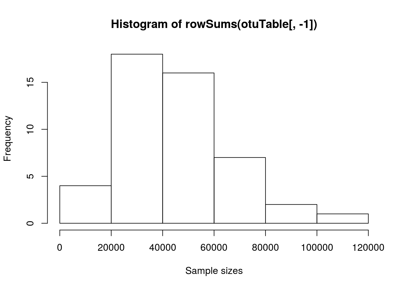
In this example, our OTU table contains 48 samples and 5381 OTUs, plus a column with the sample names in.
Now we can use microbenchmark again to compare the performance of the original rarecurve function to our faster parallel version, quickRareCurve. We will then plot the results using ggplot2. Warning: the code below will take some time to run!
library(microbenchmark)

# benchmark the two functions with 3 replicates
testResult <- microbenchmark(
  rarecurve(otuTable[, -1]),
  quickRareCurve(otuTable[, -1]),
  times = 3)
library(ggplot2)
# convert from nanoseconds to minutes by dividing
# time by 6e+10
ggplot(testResult, aes(x = expr, y = time/6e+10)) +
geom_boxplot() +
labs(x = "Function", y = "Time (minutes)") +
theme(axis.text = element_text(size = 16),
axis.title = element_text(size = 18))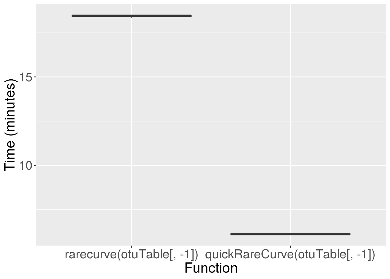
There you go, on a typical OTU table, the quickRareCurve function is far quicker, reducing the processing time from ~25 minutes to < 5 minutes. The more samples in your OTU table, and the more CPU cores available, the greater the increase in performance.