Recently, I’ve been collaborating with several colleagues on projects focussing on the microbial ecology of hydrocarbon degradation. One of the aspects we’ve been thinking about, is whether the composition of the microbial community can reflect the level of hydrocarbon exposure. As it turns out, we aren’t the first to consider this, as Mariana Lozada and colleagues came up with an “Ecological Hydrocarbon Exposure Index”, which uses the composition and structure of the microbial community to quantify the level of hydrocarbon exposure in a given environment (Lozada et al., 2014). To their credit, the authors provided R code to calculate their index in a supplementary PDF on the journal article page.

However, the original code was designed to run using a Mothur formatted taxonomy file, which is not useful for users who might prefer other taxonomy assignment pipelines. Therefore, I decided to rewrite their script into a more useful function format, that can be applied to an OTU table with any taxonomy format. The function is hosted in my GitHub based package ecolFudge, and an example of how to use this function is presented below.

# first lets import a small OTU table as an example

otus <- read.csv("example_OTU_table.csv")

# look at structure of OTU table
# note that our genus level taxonomy assignment is in "Genus" column
# and our samples all start with "THx"
str(otus)

## 'data.frame':    3488 obs. of  26 variables:
##  $ OTU              : Factor w/ 3488 levels "OTU_1","OTU_10",..: 1 1103 2205 2823 2934 3045 3156 3267 3378 2 ...
##  $ THxT1x1Bac       : int  3 3429 4653 57 1 190 555 58 0 1 ...
##  $ THxT1x2Bac       : int  1 24761 8476 144 11 1149 10748 628 3 19 ...
##  $ THxT1x3Bac       : int  0 1301 511 13 0 72 101 61 1 0 ...
##  $ THxT21x1Bac      : int  9955 5 52 332 871 127 3 33 207 52 ...
##  $ THxT21x2Bac      : int  1148 51 273 1956 2237 222 18 23 144 94 ...
##  $ THxT21x3Bac      : int  4155 17 328 2427 6246 886 34 198 1632 113 ...
##  $ THxT3x1Bac       : int  3 7232 972 392 4 397 496 3002 0 19 ...
##  $ THxT3x2Bac       : int  1 10328 939 798 22 177 962 3440 1 28 ...
##  $ THxT3x3Bac       : int  1 12733 3892 1559 15 517 1960 2511 0 61 ...
##  $ THxT7x1Bac       : int  31 1583 913 3835 2841 689 253 1392 1789 726 ...
##  $ THxT7x2Bac       : int  4774 1422 614 2181 3066 352 461 1351 15 2378 ...
##  $ THxT7x3Bac       : int  2651 2689 592 6684 1862 425 210 4090 617 1226 ...
##  $ sum              : int  572326 423114 308751 239756 239329 159273 158127 152364 137010 118647 ...
##  $ Domain           : Factor w/ 1 level "Bacteria": 1 1 1 1 1 1 1 1 1 1 ...
##  $ Confidence_domain: num  1 1 1 1 1 1 1 1 1 1 ...
##  $ Phylum           : Factor w/ 37 levels "Acetothermia",..: 32 32 32 32 32 32 32 32 32 32 ...
##  $ Confidence_phylum: num  1 1 1 1 1 1 1 1 1 1 ...
##  $ Class            : Factor w/ 76 levels "Acetothermia_genera_incertae_sedis",..: 45 45 45 45 45 45 39 45 15 15 ...
##  $ Confidence_class : num  1 1 1 1 1 1 1 1 1 1 ...
##  $ Order            : Factor w/ 142 levels "Acanthopleuribacterales",..: 96 96 9 9 136 107 24 96 110 110 ...
##  $ Confidence_order : num  1 1 1 0.99 1 1 1 1 1 1 ...
##  $ Family           : Factor w/ 283 levels "Acanthopleuribacteraceae",..: 11 183 212 64 202 214 40 183 222 222 ...
##  $ Confidence_family: num  1 1 0.98 0.94 1 1 1 1 1 1 ...
##  $ Genus            : Factor w/ 878 levels "Acanthopleuribacter",..: 32 556 644 170 189 653 79 807 656 654 ...
##  $ Confidence_genus : num  1 1 0.98 0.94 1 0.97 1 1 0.48 0.99 ...

# we first need to create a vector of sample names that we wish to calculate
# the index for
samples <- grep("THx", colnames(otus), value = T)

# now we can load the ecolFudge package
# if you haven't installed it, install it using the devtools package:
# devtools::install_github("dave-clark/ecolFudge")
library(ecolFudge)

# now we simply run the index function, giving it the name of our OTU table
# the vector of sample column names, and the column with the genus level
# taxonomy assignments
sampleExposure <- ehei(otus, taxonomyCol = "Genus", sampleCols = samples)

## Calculating Ecological Hydrocarbon exposure index for 12 sample(s)

# view the results
head(sampleExposure)

##                  sample  exposure
## THxT1x1Bac   THxT1x1Bac 0.4419401
## THxT1x2Bac   THxT1x2Bac 0.3618828
## THxT1x3Bac   THxT1x3Bac 0.3674791
## THxT21x1Bac THxT21x1Bac 0.7187549
## THxT21x2Bac THxT21x2Bac 0.3846276
## THxT21x3Bac THxT21x3Bac 0.5097866

summary(sampleExposure$exposure)

##    Min. 1st Qu.  Median    Mean 3rd Qu.    Max. 
##  0.3619  0.3952  0.4759  0.4904  0.5648  0.7188

hist(sampleExposure$exposure, xlab = "Ecological hydrocarbon exposure index")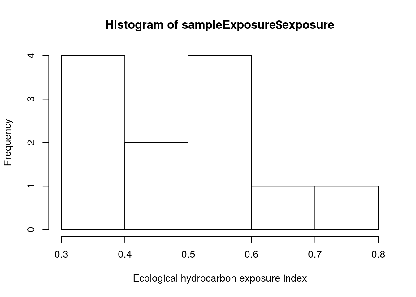

Hopefully this will be useful to any oil microbiologists out there, particularly those who are forging their own bioinformatics pipelines. As always, feel free to contact me if you have any questions/comments.

References

Lozada, M., Marcos, M.S., Commendatore, M.G., Gil, M.N. & Dionisi, H.M. (2014) The Bacterial Community Structure of Hydrocarbon-Polluted Marine Environments as the Basis for the Definition of an Ecological Index of Hydrocarbon Exposure. Microbes and Environments, ME14028.