The data.table package has become my favourite R package for all things data handling. Unlike the “tidyverse” suite of packages, the syntax is more akin to base data.frame syntax, meaning I was able to pick it up quite quickly. It is also incredibly quick, and the parallel data import/export functions (fread & fwrite) are a real gift for working with larger data tables, like OTU tables, which can contain several hundred columns, and many thousands of rows. The only thing I found data.table lacked was a function to transpose data in a convenient way.
Let me demonstrate what I mean with some examples. Let’s load a small toy dataset that is topologically similar to an OTU table (e.g. samples as cols, species abundances as rows).
# load data.table and vegan packages
library(data.table)
library(vegan)
## Loading required package: permute## Loading required package: lattice## This is vegan 2.5-4# load the Barro Colorado Island tree dataset
data(BCI)
# coerce to a data.table
# keep the rownames, as this we'll use this as a 'sample' column
bci <- as.data.table(BCI, keep.rownames = T)
# make more realistic sample names and delete old col
bci[, ":="(sampleName = paste0("sample_", rn), rn = NULL)]Now the data represent something comparable to the OTU tables I am used to working with. Species are columns, whilst each row represents a sample. However, it is common to want to work with the data in the opposite format, with samples as columns and species as rows. Intuitively, one would normally transpose the data using the t function.
transBci <- t(bci)

str(transBci)
## chr [1:226, 1:50] "0" "0" "0" "0" " 0" "0" " 2" "0" "0" "0" "25" "0" ...
## - attr(*, "dimnames")=List of 2
## ..$ : chr [1:226] "Abarema.macradenia" "Vachellia.melanoceras" "Acalypha.diversifolia" "Acalypha.macrostachya" ...
## ..$ : NULLHowever, as you can see, this causes problems. Having a sample column present in our data means that all the counts get coerced to character class when transposed. Plus, we’d have to manually set the sample row as our new column names, and then delete it from the data.
An alternate solution involves using melt and dcast functions to transpose the data…
transBci2 <- dcast(melt(bci, id.vars = "sampleName"), variable ~ sampleName)

str(transBci2)
## Classes 'data.table' and 'data.frame': 225 obs. of 51 variables:
## $ variable : Factor w/ 225 levels "Abarema.macradenia",..: 1 2 3 4 5 6 7 8 9 10 ...
## $ sample_1 : int 0 0 0 0 0 0 2 0 0 0 ...
## $ sample_10: int 1 0 0 0 0 1 2 0 0 0 ...
## $ sample_11: int 0 0 0 0 0 0 10 0 0 0 ...
## $ sample_12: int 0 0 0 0 1 1 3 0 0 2 ...
## $ sample_13: int 0 0 0 0 1 1 1 0 1 1 ...
## $ sample_14: int 0 0 0 0 0 0 4 0 0 0 ...
## $ sample_15: int 0 0 0 0 2 0 2 0 0 0 ...
## $ sample_16: int 0 0 0 0 2 0 2 0 0 3 ...
## $ sample_17: int 0 0 0 0 0 1 2 0 0 2 ...
## $ sample_18: int 0 0 0 0 1 1 0 0 0 0 ...
## $ sample_19: int 0 0 0 0 0 1 1 0 0 1 ...
## $ sample_2 : int 0 0 0 0 0 0 1 0 0 0 ...
## $ sample_20: int 0 0 0 0 0 2 2 0 0 0 ...
## $ sample_21: int 0 0 0 0 0 1 2 0 0 1 ...
## $ sample_22: int 0 0 0 0 1 0 4 0 0 4 ...
## $ sample_23: int 0 0 0 0 0 0 1 0 0 0 ...
## $ sample_24: int 0 0 0 0 2 1 0 0 0 1 ...
## $ sample_25: int 0 0 0 0 0 1 2 0 0 0 ...
## $ sample_26: int 0 0 0 0 0 0 3 0 0 0 ...
## $ sample_27: int 0 0 0 0 1 4 3 0 0 3 ...
## $ sample_28: int 0 2 0 1 0 1 2 0 0 0 ...
## $ sample_29: int 0 0 0 0 1 0 1 0 0 0 ...
## $ sample_3 : int 0 0 0 0 0 0 2 0 0 0 ...
## $ sample_30: int 0 0 0 0 14 2 6 0 0 0 ...
## $ sample_31: int 0 0 0 0 5 0 4 0 0 0 ...
## $ sample_32: int 0 1 0 0 7 0 6 0 0 0 ...
## $ sample_33: int 0 0 0 0 3 1 3 0 0 1 ...
## $ sample_34: int 0 0 1 0 3 0 5 0 0 0 ...
## $ sample_35: int 0 0 0 0 6 0 8 0 0 0 ...
## $ sample_36: int 0 0 0 0 1 0 3 0 0 0 ...
## $ sample_37: int 0 0 0 0 2 0 4 0 0 0 ...
## $ sample_38: int 0 0 0 0 6 0 2 0 0 1 ...
## $ sample_39: int 0 0 0 0 9 0 3 0 0 1 ...
## $ sample_4 : int 0 0 0 0 3 0 18 0 0 0 ...
## $ sample_40: int 0 0 1 0 7 0 3 0 0 1 ...
## $ sample_41: int 0 0 0 0 0 1 11 0 0 0 ...
## $ sample_42: int 0 0 0 0 0 0 0 0 0 0 ...
## $ sample_43: int 0 0 0 0 0 1 3 0 0 0 ...
## $ sample_44: int 0 0 0 0 4 0 4 0 0 0 ...
## $ sample_45: int 0 0 0 0 0 0 0 0 0 0 ...
## $ sample_46: int 0 0 0 0 0 0 0 0 0 0 ...
## $ sample_47: int 0 0 0 0 2 0 1 0 0 1 ...
## $ sample_48: int 0 0 0 0 1 0 3 0 0 1 ...
## $ sample_49: int 0 0 0 0 0 0 6 0 0 1 ...
## $ sample_5 : int 0 0 0 0 1 1 3 0 0 1 ...
## $ sample_50: int 0 0 0 0 1 0 2 0 0 1 ...
## $ sample_6 : int 0 0 0 0 0 0 2 1 0 0 ...
## $ sample_7 : int 0 0 0 0 0 1 0 0 0 0 ...
## $ sample_8 : int 0 0 0 0 0 0 2 0 0 0 ...
## $ sample_9 : int 0 0 0 0 5 0 2 0 0 0 ...
## - attr(*, ".internal.selfref")=<externalptr>
## - attr(*, "sorted")= chr "variable"That’s better: the sample names are now in the correct place, we have a column with the species names, and the data have remained in the correct integer class. However, whilst that code may have run quite quickly, much larger datasets can slow it down. I therefore wrote a little function based on the original transpose function to get the same result as above, but quicker!
The function is called transDT and can be found in my GitHub hosted package, ecolFudge.
# first install my package from github
library(devtools)

install_github("dave-clark/ecolFudge")

# load ecolFudge package
library(ecolFudge)

# view the transDT function
transDT
## function (dt, transCol, rowID)
## {
## newRowNames <- colnames(dt)
## newColNames <- dt[, transCol, with = F]
## transposedDt <- transpose(dt[, !colnames(dt) %in% transCol,
## with = F])
## colnames(transposedDt) <- unlist(newColNames)
## transposedDt[, rowID] <- newRowNames[newRowNames != transCol]
## return(transposedDt)
## }
## <bytecode: 0xa9ac768>
## <environment: namespace:ecolFudge>As you can see, the function takes three arguments. The first, dt, is simply the data.table you wish to transpose. The second, transCol, is the column that you wish to become your new column names. In our example, this would be the sampleName column. The third argument, rowID, is simply the name you would like to call the column with your new row identifiers (e.g. the column names in your original data). In this example, our new row identifiers are the names of the species, and so it makes sense to call this column species or something similar.
transBci3 <- transDT(bci, transCol="sampleName", rowID = "species")

# note that the species column has been placed as the last column...
str(transBci3)
## Classes 'data.table' and 'data.frame': 225 obs. of 51 variables:
## $ sample_1 : int 0 0 0 0 0 0 2 0 0 0 ...
## $ sample_2 : int 0 0 0 0 0 0 1 0 0 0 ...
## $ sample_3 : int 0 0 0 0 0 0 2 0 0 0 ...
## $ sample_4 : int 0 0 0 0 3 0 18 0 0 0 ...
## $ sample_5 : int 0 0 0 0 1 1 3 0 0 1 ...
## $ sample_6 : int 0 0 0 0 0 0 2 1 0 0 ...
## $ sample_7 : int 0 0 0 0 0 1 0 0 0 0 ...
## $ sample_8 : int 0 0 0 0 0 0 2 0 0 0 ...
## $ sample_9 : int 0 0 0 0 5 0 2 0 0 0 ...
## $ sample_10: int 1 0 0 0 0 1 2 0 0 0 ...
## $ sample_11: int 0 0 0 0 0 0 10 0 0 0 ...
## $ sample_12: int 0 0 0 0 1 1 3 0 0 2 ...
## $ sample_13: int 0 0 0 0 1 1 1 0 1 1 ...
## $ sample_14: int 0 0 0 0 0 0 4 0 0 0 ...
## $ sample_15: int 0 0 0 0 2 0 2 0 0 0 ...
## $ sample_16: int 0 0 0 0 2 0 2 0 0 3 ...
## $ sample_17: int 0 0 0 0 0 1 2 0 0 2 ...
## $ sample_18: int 0 0 0 0 1 1 0 0 0 0 ...
## $ sample_19: int 0 0 0 0 0 1 1 0 0 1 ...
## $ sample_20: int 0 0 0 0 0 2 2 0 0 0 ...
## $ sample_21: int 0 0 0 0 0 1 2 0 0 1 ...
## $ sample_22: int 0 0 0 0 1 0 4 0 0 4 ...
## $ sample_23: int 0 0 0 0 0 0 1 0 0 0 ...
## $ sample_24: int 0 0 0 0 2 1 0 0 0 1 ...
## $ sample_25: int 0 0 0 0 0 1 2 0 0 0 ...
## $ sample_26: int 0 0 0 0 0 0 3 0 0 0 ...
## $ sample_27: int 0 0 0 0 1 4 3 0 0 3 ...
## $ sample_28: int 0 2 0 1 0 1 2 0 0 0 ...
## $ sample_29: int 0 0 0 0 1 0 1 0 0 0 ...
## $ sample_30: int 0 0 0 0 14 2 6 0 0 0 ...
## $ sample_31: int 0 0 0 0 5 0 4 0 0 0 ...
## $ sample_32: int 0 1 0 0 7 0 6 0 0 0 ...
## $ sample_33: int 0 0 0 0 3 1 3 0 0 1 ...
## $ sample_34: int 0 0 1 0 3 0 5 0 0 0 ...
## $ sample_35: int 0 0 0 0 6 0 8 0 0 0 ...
## $ sample_36: int 0 0 0 0 1 0 3 0 0 0 ...
## $ sample_37: int 0 0 0 0 2 0 4 0 0 0 ...
## $ sample_38: int 0 0 0 0 6 0 2 0 0 1 ...
## $ sample_39: int 0 0 0 0 9 0 3 0 0 1 ...
## $ sample_40: int 0 0 1 0 7 0 3 0 0 1 ...
## $ sample_41: int 0 0 0 0 0 1 11 0 0 0 ...
## $ sample_42: int 0 0 0 0 0 0 0 0 0 0 ...
## $ sample_43: int 0 0 0 0 0 1 3 0 0 0 ...
## $ sample_44: int 0 0 0 0 4 0 4 0 0 0 ...
## $ sample_45: int 0 0 0 0 0 0 0 0 0 0 ...
## $ sample_46: int 0 0 0 0 0 0 0 0 0 0 ...
## $ sample_47: int 0 0 0 0 2 0 1 0 0 1 ...
## $ sample_48: int 0 0 0 0 1 0 3 0 0 1 ...
## $ sample_49: int 0 0 0 0 0 0 6 0 0 1 ...
## $ sample_50: int 0 0 0 0 1 0 2 0 0 1 ...
## $ species : chr "Abarema.macradenia" "Vachellia.melanoceras" "Acalypha.diversifolia" "Acalypha.macrostachya" ...
## - attr(*, ".internal.selfref")=<externalptr>Now let’s see whether the transDT function can be faster than the dcast/melt method…
library(microbenchmark)

speedTest <- microbenchmark(
  transDT(bci, transCol = "sampleName", rowID = "species"),
  dcast(melt(bci, id.vars = "sampleName"), variable ~ sampleName),
  times = 50)

# rename factor levels to neaten up results plot
speedTest$expr <- factor(speedTest$expr,
  levels = levels(speedTest$expr),
  labels = c("transDT", "dcast/melt"))

boxplot(time/1000 ~ expr,
  data = speedTest,
  ylab = expression(paste("Time (", mu, "S)")),
  xlab = "Method")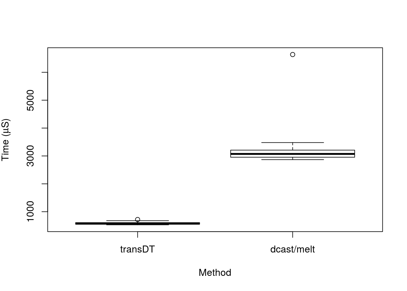
There you have it, transDT gives us the same result, but in a fraction of the time compared to the dcast/melt method, even on a relatively small dataset. I hope this is useful to other R users other than myself, if you have any questions, do get in touch!